Global measurement of tropospheric wind has been widely recognized as potentially the most significant contribution of satellite remote sensing to existing global meteorological observations ("Call for Winds"). Most of the world's oceans are largely devoid of accurate wind measurements, a deficiency that can best be addressed from space. The deployment of such an instrument would provide the capability to address many of the key issues facing the Earth Sciences in the 21st century (e.g., hydrologic and biogeochemical cycles, planetary scale dynamics, atmospheric-oceanic heat transport). Equally important, it would provide critical wind information for improved operational weather forecasting, and for safe, efficient, and effective military and commercial aviation operations. Direct measurement of horizontal wind vectors in clear air has been demonstrated using lidar from the ground and from aircraft, based on determination of the wind-induced Doppler shift in the backscatter signal.

The global tropospheric wind sounder mission requirements are listed below in Table 1. Two sets of requirements are provided; the first set are operational prototype threshold requirements and the second set are operational mission threshold requirements which meet NOAA’s operational mission requirements. These requirements are the results of discussions over the past several years with input from both the operational and research communities. The requirements listed here are threshold requirements, which are the minimal data specifications for a system to benefit both the earth science and the operational weather forecasting communities.

1. Regional
2. Global
3. For lidar systems only

General Notes:

1. Assume a baseline of at least two perspectives within a Resolution Volume (RV).
2. A single perspective is assumed if the range of azimuths for shots being accumulated or averaged is less than 10 degrees.
3. Total Observation Error (TOE) must include lidar instrument errors; pointing knowledge errors, pulse scale wind variance and sampling errors due to shot pattern and the variance of the winds within the RV. See Appendix 2 for further explaination.
4. At this time, the potential relative merits of Doppler Wind Lidars (DWLs) that only sense winds in the cloud free mid/upper troposphere vs. DWLs that sense winds within the Planetary Boundary Layer (PBL), aerosol rich areas of the mid/upper troposphere, and clouds are awaiting the execution of Observing System Simulation Experiments(OSSEs) at NOAA/NCEP. The impact of data voids and selective targeting of DWL observations are also being studied.
5. Product latency (i.e., maximum time period between actual space-based measurements and delivery of processed data) should be 2 hours or less.
6. Global coverage assumes a sun-synchronous orbit. Equator crossing time unspecified.

Cluster Patterns: "Cluster" denotes a pattern of lidar shots that are nearly co-located (~DX =10-20 km) to achieve a single line-of-sight measurement by averaging or accumulating multiple samples with the same geometric perspective (i.e., fixed azimuth and elevation angles). In this case, "cluster" further implies that a cluster of forward shots is nearly collocated with a cluster of aft shots. A pair of forward and aft clusters constitutes the domain of a "preferred wind vector product" (see notes). The nominal distance between cluster pairs measured in kilometers is expected to be at least the threshold horizontal resolution.

Vertical Resolution: The vertical distance (DZ) over which raw lidar signal can be processed to produce a single LOS wind estimate. In clouds, the vertical extent of usable lidar signal will be determined by the extinction ratio. In the PBL, 250 m is desirable but it is expected that in low backscatter situations, a greater depth of return may need to be used to obtain a meaningful LOS estimate. Thus the design resolution should be thought of as being applicable to high SNR situations.

Appendix 2. Total Observation Error

s_o² = error variance of observations (as used by model) - difference between observed value and the true value defined as the average value of the parameters within a radius 1/2 D. [D is either the utility grid resolution or the distance between data clusters. The utility grid is aligned with the satellite track and is used to aggregate shots to produce single LOS estimates.]

s_m² = variance (mostly uncorrelated) in the horizontally projected LOS measure that is due to the combined effects of instrument errors, signal processing uncertainties and atmospheric turbulence/shear on all scales less than 2*l (l = processing range gate).

s_c² = variance (mostly correlated) in the horizontal wind field (single component) on all scales 2*l < l < 2*L (L is the length scale for any shot clustering).

s_a² = variance in the horizontal wind (single component) on all scales 2L < l < 2D within "area of regard".

s_t² = s_m² + s_c² + s_a² = total variance in the horizontal wind in a single direction on all scales

N_a = number of shots or clusters of shots that are effective in reducing the s_a² wind variance.

N_a · N_c = N_T

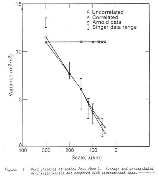
Based upon correlated variance distribution in Figure 1, s_c² and s_a² are computed as follows:

s_c² = (14/400) * 2 * (L-l)

s_a² = (14/400) * 2 * (D-L)

To minimize s_o²:

s_m² = 2 P = 1 (high SNR region)

so = 3.48 m/s

so = .89 m/s